ADVANCED DATA STRUCTURES

Binary Search Tree

Binary search tree is a data structure that quickly allows us to maintain a sorted list of numbers.

• It is called a binary tree because each tree node has maximum of two children.

• It is called a search tree because it can be used to search for the presence of a number in O(log(n)) time.

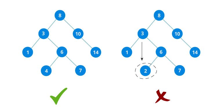
The properties that separates a binary search tree from a regular binary tree is

1. All nodes of left subtree are less than root node

2. All nodes of right subtree are more than root node

3. Both subtrees of each node are also BSTs i.e. they have the above two properties

A tree having a right subtree with one value smaller than the root is shown to demonstrate that it is not a valid binary search tree

The binary tree on the right isn't a binary search tree because the right subtree of the node "3" contains a value smaller that it.

There are two basic operations that you can perform on a binary search tree:

1. Check if number is present in binary search tree

The algorithm depends on the property of BST that if each left subtree has values below root and each right subtree has values above root.

If the value is below root, we can say for sure that the value is not in the right subtree; we need to only search in the left subtree and if the value is above root, we can say for sure that the value is not in the left subtree; we need to only search in the right subtree.

Algorithm:

If root == NULL 
    return NULL;
If number == root->data 
    return root->data;
If number < root->data 
    return search(root->left)
If number > root->data 
    return search(root->right)

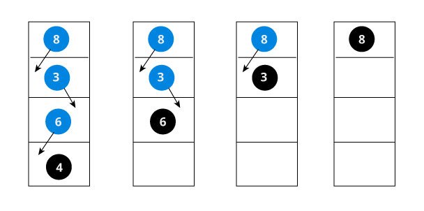
Let us try to visualize this with a diagram.

binary search tree downward recursion step involves searching in left subtree or right subtree depending on whether the value is less than or greater than the root

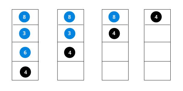
If the value is found, we return the value so that it gets propogated in each recursion step as shown in the image below.

If you might have noticed, we have called return search(struct node*) four times. When we return either the new node or NULL, the value gets returned again and again until search(root) returns the final result.

if the value is found in any of the subtrees, it is propagated up so that in the end it is returned, otherwise null is returned

If the value is not found, we eventually reach the left or right child of a leaf node which is NULL and it gets propagated and returned.

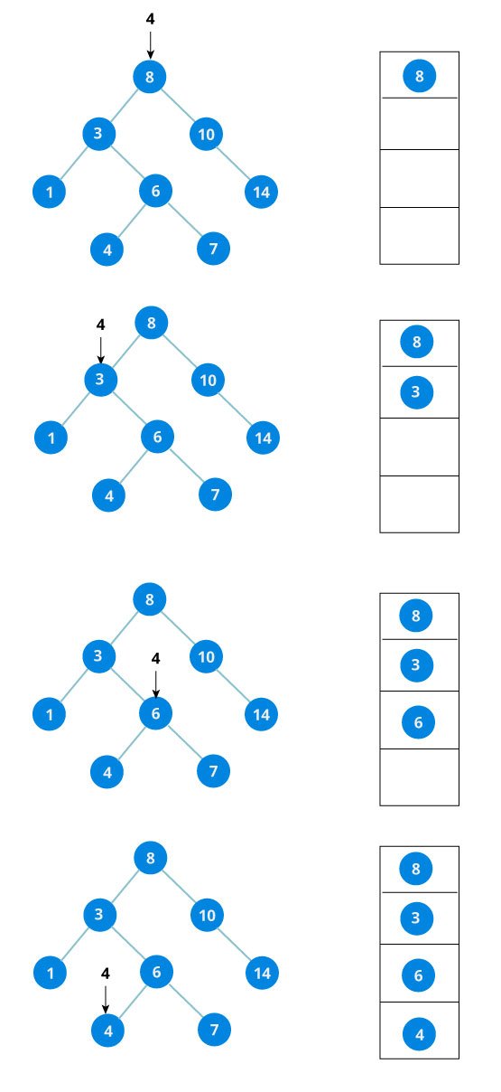
2. Insert value in Binary Search Tree(BST)

Inserting a value in the correct position is similar to searching because we try to maintain the rule that left subtree is lesser than root and right subtree is larger than root.

We keep going to either right subtree or left subtree depending on the value and when we reach a point left or right subtree is null, we put the new node there.

Algorithm:

If node == NULL 
    return createNode(data)
if (data < node->data)
    node->left  = insert(node->left, data);
else if (data > node->data)
    node->right = insert(node->right, data);  
return node;

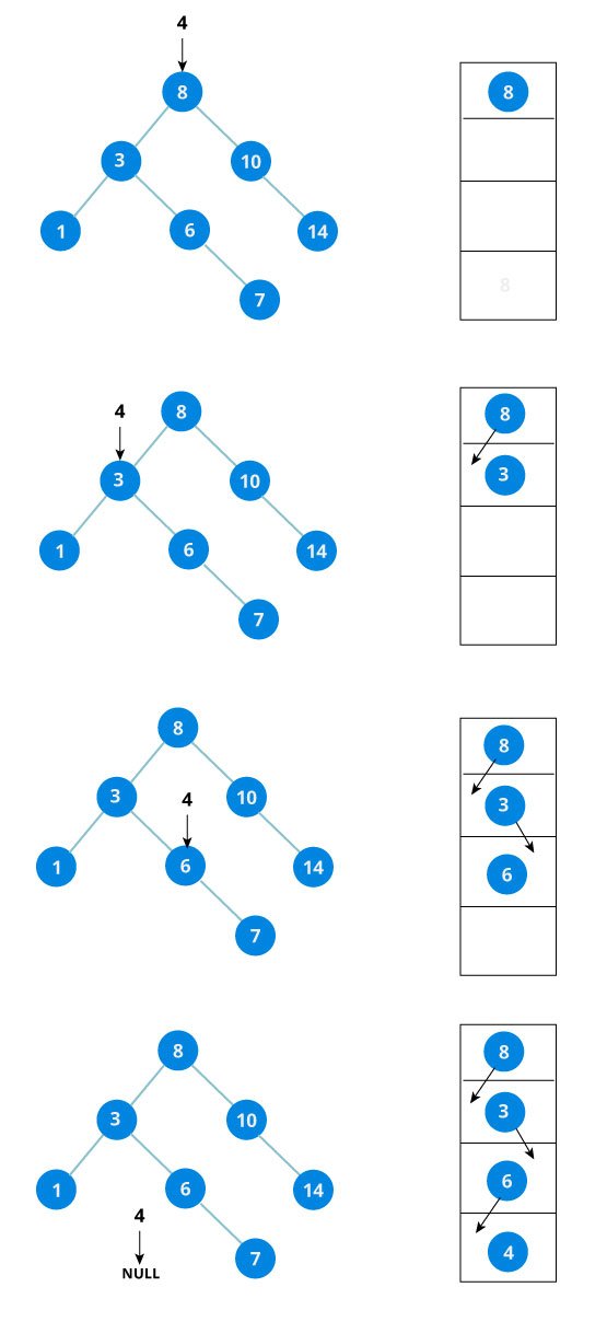
The algorithm isn't as simple as it looks. Let's try to visualize how we add a number to an existing BST.

steps that show how the algorithm of insertion to maintain a tree as binary search tree works

We have attached the node but we still have to exit from the function without doing any damage to the rest of the tree. This is where the return node; at the end comes in handy. In the case of NULL, the newly created node is returned and attached to the parent node, otherwise the same node is returned without any change as we go up until we return to the root.

This makes sure that as we move back up the tree, the other node connections aren't changed.

image showing the importance of returning the root element at the end so that the elements don't lose their position during upward recursion step.

The complete code for Binary Search Tree insertion and searching in C programming language is posted below:

#include<stdio.h>
#include<stdlib.h>
  
struct node
{
    int data;
    struct node* left;
    struct node* right;
};

struct node* createNode(value){
    struct node* newNode = malloc(sizeof(struct node));
    newNode->data = value;
    newNode->left = NULL;
    newNode->right = NULL;

    return newNode;
}
  
  
struct node* insert(struct node* root, int data)
{
    if (root == NULL) return createNode(data);

    if (data < root->data)
        root->left  = insert(root->left, data);
    else if (data > root->data)
        root->right = insert(root->right, data);   
 
    return root;
}

void inorder(struct node* root){
    if(root == NULL) return;
    inorder(root->left);
    printf("%d ->", root->data);
    inorder(root->right);
}


int main(){
    struct node *root = NULL;
    root = insert(root, 8);
    insert(root, 3);
    insert(root, 1);
    insert(root, 6);
    insert(root, 7);
    insert(root, 10);
    insert(root, 14);
    insert(root, 4);

    inorder(root);
}

The output of the program will be

1 ->3 ->4 ->6 ->7 ->8 ->10 ->14 ->

Graph Data Stucture

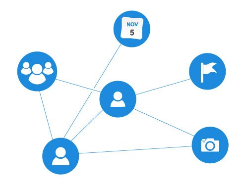
A graph data structure is a collection of nodes that have data and are connected to other nodes.

Let's try to understand this by means of an example. On facebook, everything is a node. That includes User, Photo, Album, Event, Group, Page, Comment, Story, Video, Link, Note...anything that has data is a node.

Every relationship is an edge from one node to another. Whether you post a photo, join a group, like a page etc., a new edge is created for that relationship.

graph data structure explained using facebook's example. Users, groups, pages, events etc. are represented as nodes and their relationships - friend, joining a group, liking a page are represented as links between nodes

All of facebook is then, a collection of these nodes and edges. This is because facebook uses a graph data structure to store its data.

More precisely, a graph is a data structure (V,E) that consists of

• A collection of vertices V

• A collection of edges E, represented as ordered pairs of vertices (u,v)

a graph contains vertices that are like points and edges that connect the points

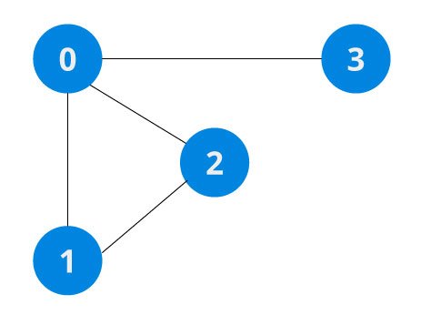
In the graph,

V = {0, 1, 2, 3}
E = {(0,1), (0,2), (0,3), (1,2)}
G = {V, E}

Graph Terminology

• Adjacency: A vertex is said to be adjacent to another vertex if there is an edge connecting them. Vertices 2 and 3 are not adjacent because there is no edge between them.

• Path: A sequence of edges that allows you to go from vertex A to vertex B is called a path. 0-1, 1-2 and 0-2 are paths from vertex 0 to vertex 2.

• Directed Graph: A graph in which an edge (u,v) doesn't necessary mean that there is an edge (v, u) as well. The edges in such a graph are represented by arrows to show the direction of the edge.

Graph Representation

Graphs are commonly represented in two ways:

1. Adjacency Matrix

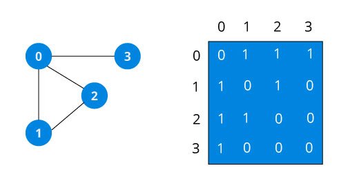
An adjacency matrix is 2D array of V x V vertices. Each row and column represent a vertex.

If the value of any element a[i][j] is 1, it represents that there is an edge connecting vertex i and vertex j.

The adjacency matrix for the graph we created above is

graph adjacency matrix for sample graph shows that the value of matrix element is 1 for the row and column that have an edge and 0 for row and column that don't have an edge

Since it is an undirected graph, for edge (0,2), we also need to mark edge (2,0); making the adjacency matrix symmetric about the diagonal.

Edge lookup(checking if an edge exists between vertex A and vertex B) is extremely fast in adjacency matrix representation but we have to reserve space for every possible link between all vertices(V x V), so it requires more space.

class Graph(object):
    def __init__(self, size):
        self.adjMatrix = []
        for i in range(size):
            self.adjMatrix.append([0 for i in range(size)])
        self.size = size

    def addEdge(self, v1, v2):
        if v1 == v2:
            print("Same vertex %d and %d" % (v1, v2))
        self.adjMatrix[v1][v2] = 1
        self.adjMatrix[v2][v1] = 1

    def removeEdge(self, v1, v2):
        if self.adjMatrix[v1][v2] == 0:
            print("No edge between %d and %d" % (v1, v2))
            return
        self.adjMatrix[v1][v2] = 0
        self.adjMatrix[v2][v1] = 0

    def containsEdge(self, v1, v2):
        return True if self.adjMatrix[v1][v2] > 0 else False

    def __len__(self):
        return self.size
        
    def toString(self):
        for row in self.adjMatrix:
            for val in row:
                print('{:4}'.format(val)),
            print
        
def main():
        g = Graph(5)
        g.addEdge(0, 1);
        g.addEdge(0, 2);
        g.addEdge(1, 2);
        g.addEdge(2, 0);
        g.addEdge(2, 3);
    
        g.toString()
            
if __name__ == '__main__':
   main()

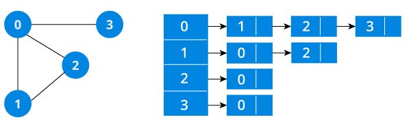
2. Adjacency List

An adjacency list represents a graph as an array of linked list.

The index of the array represents a vertex and each element in its linked list represents the other vertices that form an edge with the vertex.

The adjacency list for the graph we made in the first example is as follows:

adjacency list representation represents graph as array of linked lists where index represents the vertex and each element in linked list represents the edges connected to that vertex

An adjacency list is efficient in terms of storage because we only need to store the values for the edges. For a graph with millions of vertices, this can mean a lot of saved space.

Adjacency List Python

There is a reason Python gets so much love. A simple dictionary of vertices and its edges is a sufficient representation of a graph. You can make the vertex itself as complex as you want.

graph = {'A': set(['B', 'C']),
         'B': set(['A', 'D', 'E']),
         'C': set(['A', 'F']),
         'D': set(['B']),
         'E': set(['B', 'F']),
         'F': set(['C', 'E'])}

Graph Operations

The most common graph operations are:

• Check if element is present in graph

• Graph Traversal

• Add elements(vertex, edges) to graph

• Finding path from one vertex to another